Resolution calculation with Instrument class
In this tutorial usage examples of :py:class`.Instrument` for both Triple Axis and Time of Flight instruments will be given. While the Triple Axis instrument features are stable, Time of Flight instrumentation is still under development, and there could be minor changes and major additions going forward.
Triple Axis Instruments
The following are examples on the usage of the Instrument class with instrument_type="tas", which instances a TripleAxisInstrument object, used to define a triple-axis spectrometer instrument configuration and calculate the resolution in reciprocal lattice units for a given sample at a given wave-vector \(q\). The next sections of this tutorial will cover the utilization of both Cooper-Nathans and Popovici calculation methods. The tutorial for Time of Flight spectrometers follows these sections.
Instrument Configuration
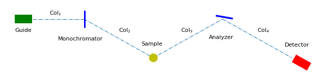
First, we will begin by defining an generic triple-axis spectrometer instrument configuration that we will use for this example.
(Source code, png, hires.png, pdf)

For the Cooper-Nathans calculation only a rudimentary set of information is required to estimate the resolution at a given \(q\). Namely, the fixed energy (incident or final), the relevant (horizontal) collimations (Col\(_n\)), and the monochromator and analyzer crystal types (or \(\tau\), if the crystal type is not included in this software). In this case we will use the following values:
>>> efixed = 14.7
>>> hcol = [40, 40, 40, 40]
>>> ana = 'PG(002)'
>>> mono = 'PG(002)'
The rest of the required information are all dependent on the sample configuration.
Note
Many settings have default values, that don’t need to be changed for the resolution calculation to function, but will provide more accuracy if assigned appropriate values.**
Sample Configuration
Defining the sample using the Sample class is simple. In this example we define an arbitrary sample with no given sample mosaic.
>>> from neutronpy import Sample
>>> sample = Sample(6, 7, 8, 90, 90, 90, u=[1, 0, 0], v=[0, 1, 0])
where the inputs for Sample are a, b, c, alpha, beta, gamma, and mosaic, respectively, and u and v are the orientation vectors in reciprocal lattice units. In this case the sample is oriented in the (h, k, 0)-plane
Initializing the Instrument
Once the sample is defined and information about the instrument collected we can formally define the instrument using Instrument and the variables that we have already assigned above.
>>> from neutronpy import Instrument
>>> EXP = Instrument(efixed, sample, hcol, ana=ana, mono=mono)
There are a great deal more settings available than are used here; see Instrument documentation.
Calculating the resolution
To calculate the resolution we need to define at which \(q=[h,k,l,\hbar\omega]\) we want the resolution to be calculated. There are several ways that we can go about doing this. The simplest situation is if the resolution is desired at only one point in reciprocal space, e.g. [1, 0, 0, 0], i.e. (1, 0, 0) at zero energy transfer:
>>> q = np.array([1, 0, 0, 0])
More positions can be easily added; e.g. if we wanted to add (0.5, 0.5, 0) at 0 meV, and (0.5, 0., 0.5) at 8~meV, our q would have the structure:
>>> q = np.array([[1, 0.5, 0.5], [0, 0.5, 0], [0, 0, 0.5], [0, 0, 8]])
We will use this second q to calculate the resolution.
Note
We use np.array() here to allow us to use ‘fancy indexing’, which will simplify using slices of q later.
Resolution parameters
To calculate the resolution parameters, without needing projections or plots, one may use calc_resolution:
>>> EXP.calc_resolution(q)
The resulting resolution parameters, \(R_0\) and \(\mathbf{R}_M\), are saved in the EXP variable and can be accessed by
>>> RMS = EXP.RMS
>>> R0 = EXP.R0
The resolution matrix here is the full matrix, over four dimensional space N (4 \(\times\) 4) matrices, with shape (4, 4, N) (N=3 in our case). Alternatively, it is possible to extract more immediately useful parameters, i.e. projections or slices in the plane of interest using get_resolution_params.
We can get projections or slices in the x-y, x-e or y-e planes (see get_resolution_params documentation for all possible keywords); the z-plane is not accessible due to the nature of the sample orientation and is integrated out. In this case we will extract the resolution parameters for the projection into the \(Q_x Q_y\) plane for the first q, i.e. [1,0,0,0]:
>>> R0, RMxx, RMyy, RMxy = EXP.get_resolution_params(q[:, 0], 'QxQy', mode='project')
RMxx and RMyy are the diagonals of the resolution matrix, RMxy is the off-diagonals, and R0 is the pre-factor. An error will be thrown if a q that was not previously calculated is given.
Resolution ellipses
The resolution ellipses are calculated when calc_projections is called, and can be accessed using calc_projections, which is a dictionary with the keys QxQy, QxQySlice, QxW, QxWSlice, QyW, and QyWSlice, providing x and y values.
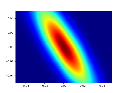
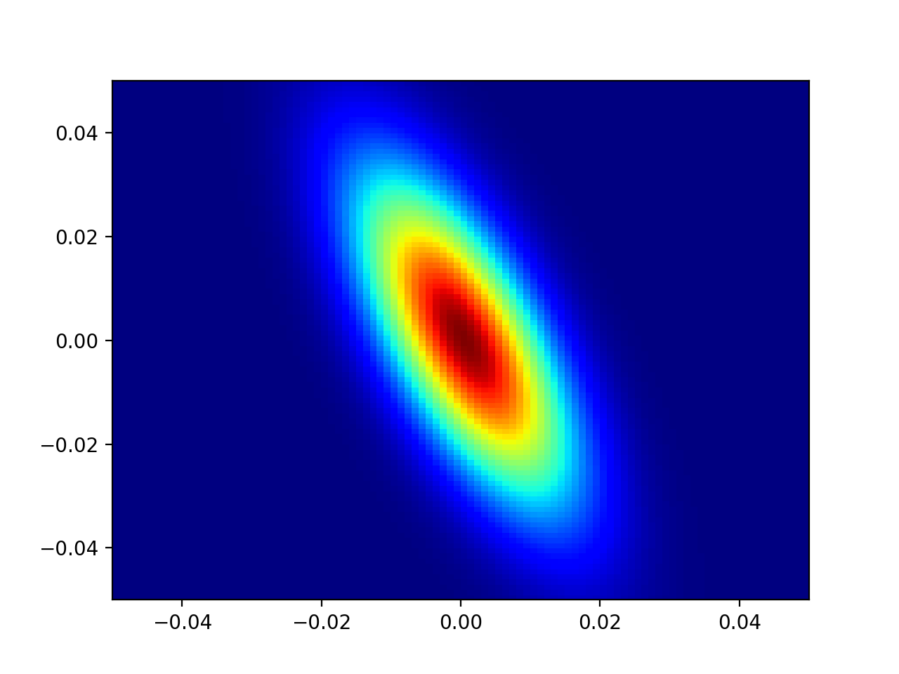
The following is an example of a resolution calculation using the Cooper-Nathans method (for a projection in the \(Q_x Q_y\) plane), with resolution ellipses (projection (filled) and slice (dashed)) overlaid, using the settings we have used in this example.
(Source code, png, hires.png, pdf)

Popovici calculation
All of the previous sections are still relevant and are necessary for the Popovici method of resolution calculation, but more details about the instrument are required, and the Popovici method must be enabled. The most essential properties that need to be defined are the distances between each major element of the instrument, namely, guide-to-monochromator, monochromator-to-sample, sample-to-analyzer, and analyzer-to-detector. These distances are assigned to the arms property in the above order:
>>> EXP.arms = [1560, 600, 260, 300]
Once this variable is set we can enable the Popovici method and recalculate the resolutions:
>>> EXP.method=1
>>> EXP.calc_resolution(q)
Note
Like with the Cooper-Nathans method above, many of these settings have default values, that don’t need to be changed for the resolution calculation to function, but will provide more accuracy if assigned appropriate values.
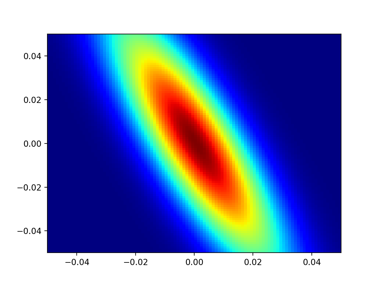
The following is an example of a resolution calculation using the Popovici method (for a projection in the \(Q_x Q_y\) plane), with resolution ellipses (projection (filled) and slice (dashed)) overlaid, using the settings used in this example.
(Source code, png, hires.png, pdf)

Plotting
Simple Plotting of Resolution Ellipses
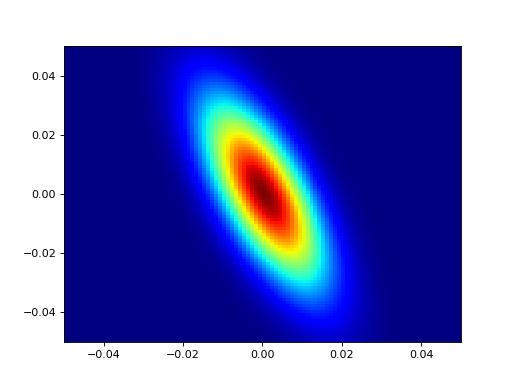
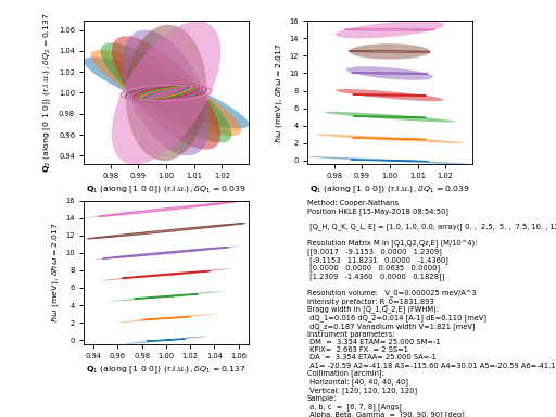
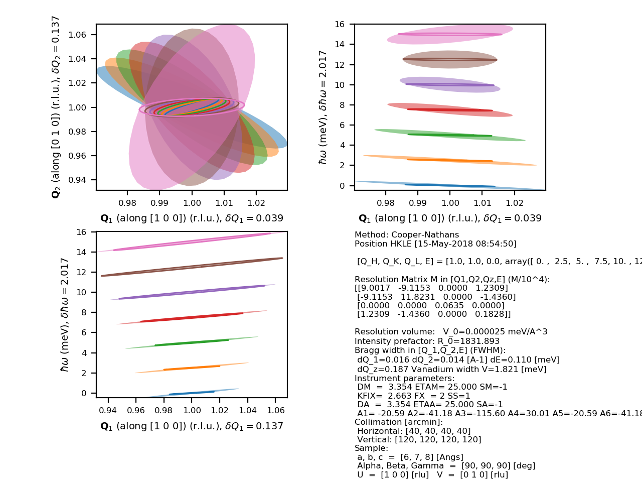
To see a simple plot of the resolution ellipses in the \(Q_x Q_y\), \(Q_x W\) and \(Q_y W\) zones the plot_projections method may be used. This will also display instrument setup parameters and other useful information such as Bragg widths.
A very simple plot for the default instrument, containing resolution ellipses for several different energies at may be obtained with these commands
>>> from numpy import linspace
>>> EXP = Instrument()
>>> EXP.plot_projections([1., 1., 0., linspace(0, 15, 7)])
(Source code, png, hires.png, pdf)

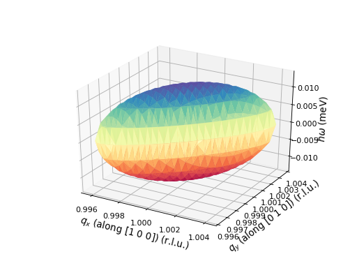
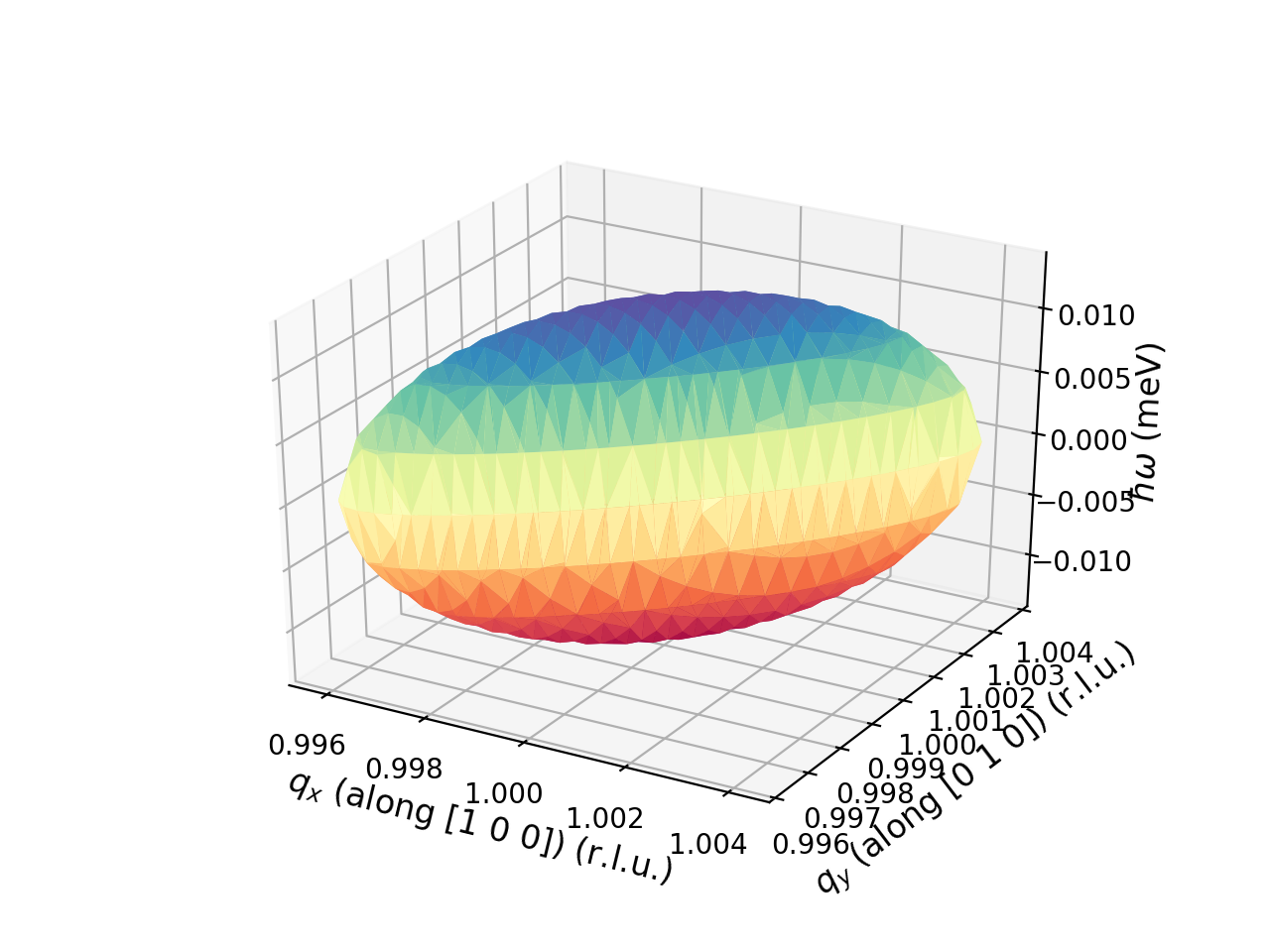
Simple Plotting of the 3D Resolution Ellipsoid
To see a simple plot of the resolution ellipsoid in the \(Q_x Q_y W\) zone the plot_ellipsoid method can be used.
>>> EXP = Instrument()
>>> EXP.plot_ellipsoid([1,1,0,0])
(Source code, png, hires.png, pdf)

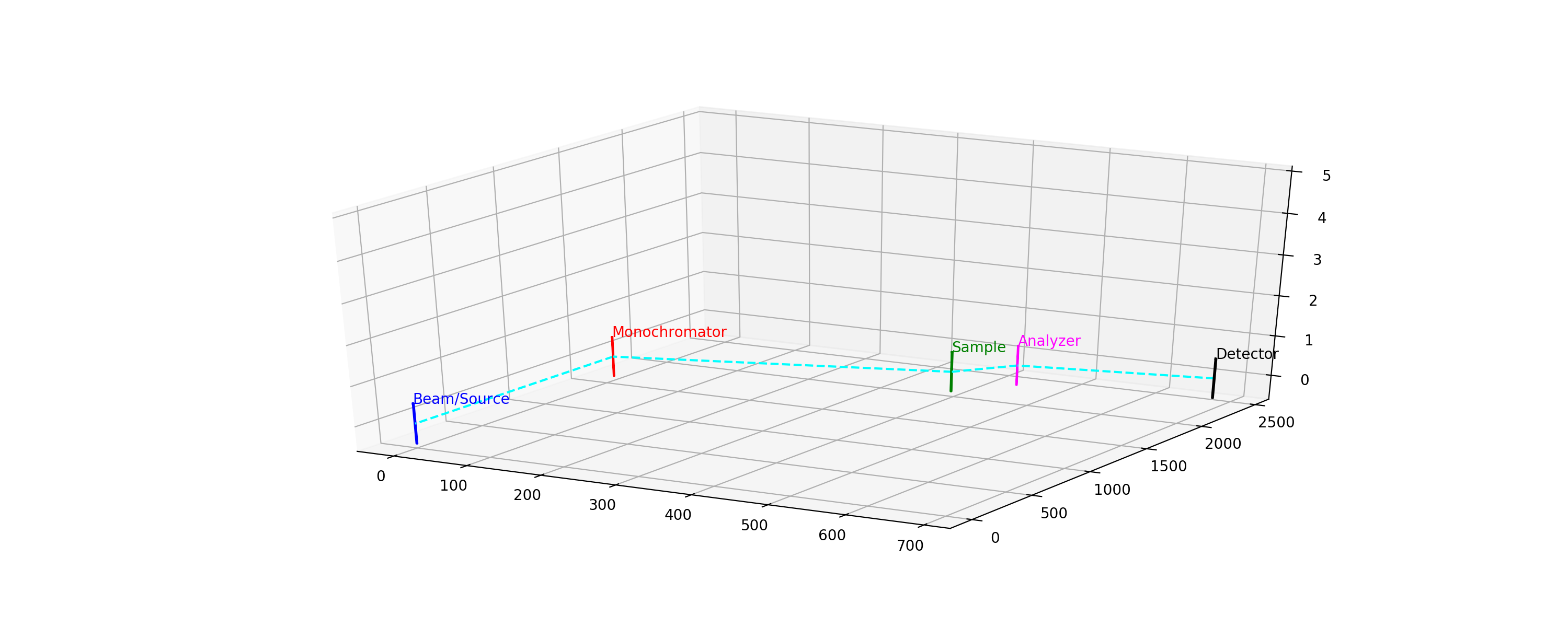
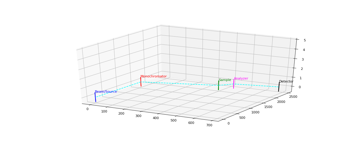
Plotting of the Instrument setup for a given (Q,W)
To see a plot of the instrument setup using the angles required for a given \((Q, W)\) the plot_instrument method can be used.
>>> EXP = Instrument()
>>> EXP.plot_instrument([1,1,0,0])
(Source code, png, hires.png, pdf)
Time of Flight spectrometers
The follow sections of this tutorial cover the use of Instrument with instrument_type="tof", which instances a TimeOfFlightInstrument object used to define a Time of Flight spectrometer configuration for resolution calculations. The resolution calculation is performed using the “Violini method”, translated from “A method to compute the covariance matrix of wavevector-energy transfer for neutron time-of-flight spectrometers” by Violini et al., Nuclear Instruments and Methods in Physics Research A 736 (2014) 31-39. DOI: 10.1016/j.nima.2013.10.042.
Instrument Configuration
Each TOF spectrometer object will include an incident Energy object, two Chopper objects, two Guide objects, a Detector object, and a Sample object.
Building a sample
Samples use the same syntax as demonstrated above in the Triple Axis sections
>>> from neutronpy import Sample
>>> sample = Sample(4, 4, 4, 90, 90, 90, u=[1, 0, 0], v=[0, 1, 0], distance=3600)
Note that distance is also included, and is a mandatory kwarg for TOF instruments. Also note that a mosaic and vmosaic are used during the resolution calculation to estimate the resolution input parameters, and therefore if none is specified, 60 min is assumed for both.
The Sample object will allow calculation of sigma_l_sd (the path-length uncertainty between the sample and the detector), and sigma_theta and sigma_phi (the uncertainties in the scattering angles).
Choppers
Chopper objects are the first of the new components for Time of Flight instruments. Each chopper has a frequency at which it spins, a distance from the neutron source, and an opening of a particular size, which can be defined in several different ways. Note that the source position is not absolutely important, just the distances between the choppers, but you will typically get the information about the instrument in this format, thus this specification. A typical chopper with a set angular acceptance in degrees can be defined by
>>> from neutronpy.instrument import Chopper
>>> chopper1 = Chopper(0, 60, 30, "disk", 10)
This first chopper is known as the “P chopper”, and is typically much more coarse than the second chopper, which is known as the “M chopper”:
>>> chopper2 = Chopper(1600, 240, 30, "disk, 8)
This defines both of our choppers, which will be passed in a list:
>>> choppers = [chopper1, chopper2]
These objects will help TimeOfFlightInstrument calculate the values tau_p and tau_m (the time resolution of each of the choppers), l_pm and l_ms (the distance between the two choppers and between the M chopper and sample).
Guides
Next, the Guide objects need to be defined by specifying the length, height, width, and m value.
>>> from neutronpy.instrument import Guide
>>> guide1 = Guide(2, 1600, 30, 30)
>>> guide2 = Guide(2, 2000, 30, 30)
>>> guides = [guide1, guide2]
These objects will help TimeOfFlightInstrument calculate sigma_l_pm and sigma_l_ms (path-length uncertainties between the P and M choppers and the M chopper and the sample), and sigma_theta_i and sigma_phi_i (the uncertainty in the in-plane and out-of-plane incident angles of the neutrons on the sample).
Detector
Finally, we must specify the :py:class`.Detector` object, specifying the shape (either spherical or cylindrical), width and height in degrees, radius in cm, horizontal pixels (given in angular acceptance of arc minutes), number of detector pixels in the vertical direction, and the time binning of the detector in microseconds. Detectors require by far the most information for the calculation.
>>> from neutronpy.instrument import Detector
>>> detector = Detector("cylindrical", [-120, 120], [-20, 20], 300, 30, 8, 0.1)
Initializing the instrument
Now that we have defined all of our components we can initialize the instrument via Instrument. Specifying ei can be done with either Energy or with a float.
>>> from neutronpy import Instrument
>>> instr = Instrument(instrument_type="tof", ei=3, choppers=choppers, guides=guides, detector=detector, sample=sample)
Alternatively it is possible to build the default instrument and individually specify the necessary lengths and uncertainties. All of the following are the necessary values, but keep in mind to change the default sample as well.
>>> instr = Instrument(instrument_type="tof")
>>> instr.ei.energy = 3.0
>>> instr.detector.shape = "cylindrical"
>>> instr.tau_p = 80.0
>>> instr.tau_m = 20.0
>>> instr.tau_d = 0.1
>>> instr.l_pm = 1600
>>> instr.l_ms = 200
>>> instr.l_sd = 300
>>> instr.theta_i = 0.0
>>> instr.phi_i = 0.0
>>> instr.sigma_l_pm = 12.0
>>> instr.sigma_l_ms = 2.0
>>> instr.sigma_l_sd = 0.5
>>> instr.sigma_theta_i = 0.5
>>> instr.sigma_theta = 0.1
>>> instr.sigma_phi_i = 0.5
>>> instr.sigma_phi = 0.2
Resolution calculation
Calculating the resolution at a particular position Q and energy transfer W works very similarly to that shown above for Triple Axis Spectrometers. In fact, the methods for calculating projections and ploting are completely shared between TripleAxisInstrument and :py:class`.TimeOfFlightInstrument`. To calculate resolution at [1, 1, 0, 0]
>>> instr.calc_resolution([1, 1, 0, 0])
This will result in R0, RM and RMS attributes in instr, which hold the same meanings as for Triple Axis Spectrometer resolution calculations.
Projections can be generated and accessed in the same way as explained above for Triple Axis Spectrometers, as can plotting. Convolution methods are the only exceptions to this.
File IO
File IO is not yet fully supported for Time of Flight spectrometers.